Climate changes have been a concern for scientists for a long time and have been the primary cause of forest fires. Forest fires are uncontrolled that occur naturally in nature. Sometimes it gets severed due to climatic changes. Forest fires are considered one of the most common threats in a forested environment.
They pose a warning to the forest’s vegetation and biodiversity. Forest fires that are unplanned and unexpected are the cause of forest degradation but controlled fire to manage and restrict the spread of forest fires is an action that helps to improve the forest. Forest fires result in an environmental threat.
Below points gives the full explanation-
1. The rise in temperature leads to dry conditions in forests, and mild snow leads to the burning of forests.
2. It makes it further drier and results in the loss of vegetation that acts as fuel for the burn of the forest.
3. It leads to an increase in CO2 concentration in the atmosphere that further increases the temperature.
CSV files downloaded from the website
Forest fires in Europe (europa.eu)
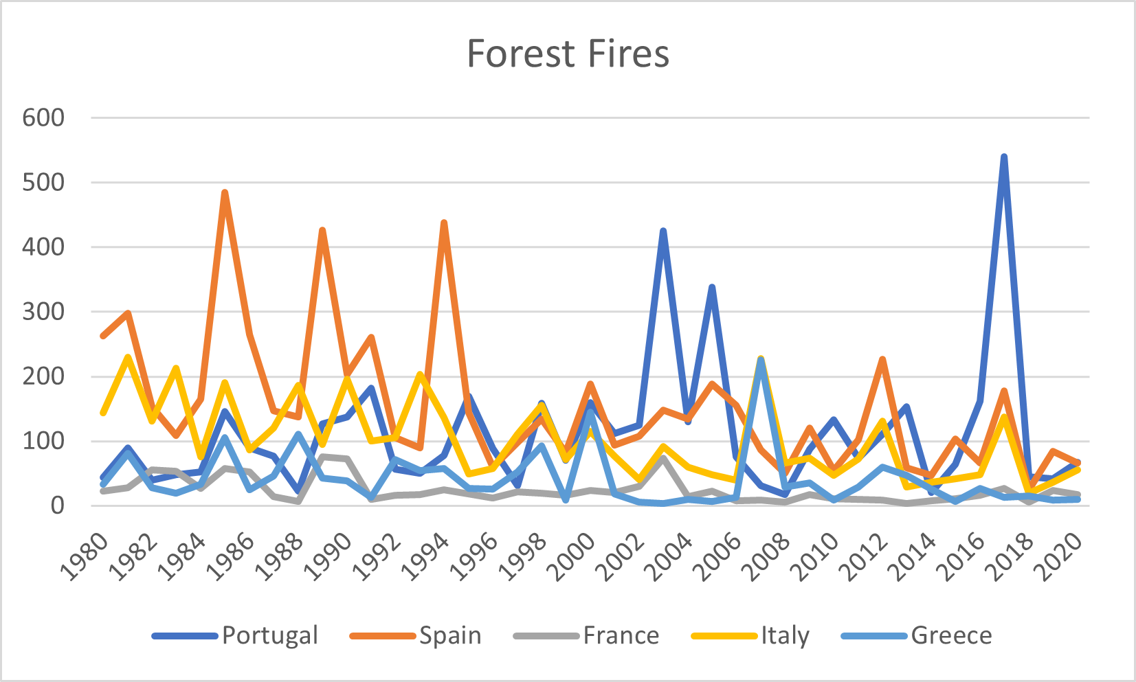
From the graph, it’s clear that some preventive measures have worked so far since 1980; however, in upcoming years, drought and heatwaves have increased in the central and northern areas of Europe, making them prone to fires.
.png)
Total Wildfires –
Total Wildfires and Acres Burned (nifc.gov)
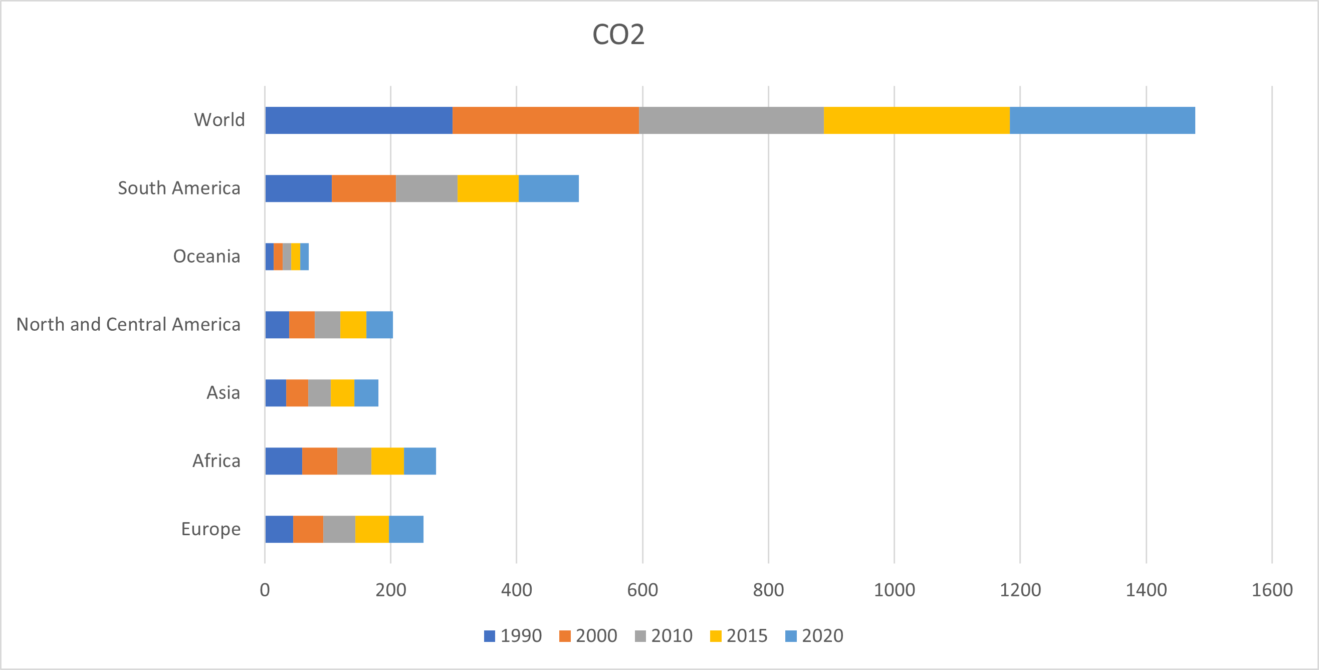
Objective
The main motive of the article is to show with the help of Auto-regressive Integrated Moving Average (ARIMA) that in the upcoming future, carbon dioxide is increasing and is a threat to the environment.
Time Series Analysis
We can download the data from – GitHub – aster28/Climate.
We will be using Google colab instead of jupyter notebook.
#Import the libraries
import numpy as np
import pandas as pd  import matplotlib.pyplot as plt %matplotlib inline  import math from keras.models import Sequential from keras.layers import Dense from keras.layers import LSTM from sklearn.preprocessing import MinMaxScaler from sklearn.metrics import mean_squared_error from sklearn.metrics import mean_absolute_error
from sklearn.model_selection import train_test_split
import seaborn as sns from IPython.display import SVG from keras.utils.vis_utils import model_to_dot  import itertools import warnings warnings.filterwarnings('ignore')

df1=pd.read_csv('Climate_Change.csv')
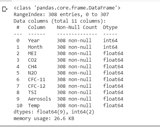
df1.info()
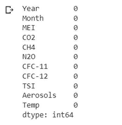
df1.isna().sum()
years = df1[‘Year’].unique()
# Draw Plot
fig, axes = plt.subplots(1, 2, figsize=(35,7), dpi= 80)
sns.boxplot(x=’Year’, y=’Temp’, data=df1, ax=axes[0])
sns.boxplot(x=’Month’, y=’Temp’, data=df1.loc[~df1.Year.isin([1983, 2008]), :])
# Set Title
axes[0].set_title(‘Year-wise Box Plot)’, fontsize=18);
axes[1].set_title(‘Month-wise Box Plot)’, fontsize=18)
plt.show()
.png)
df1[‘Date’] = df1[‘Year’].apply(str) + “-” +df1[‘Month’].apply(str)
df1.drop(['Year','Month'], axis=1, inplace=True)
df1
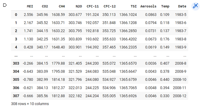
df1.set_index(‘Date’,inplace=True)
df1.head()
df1.shape
(308,9)
df1.plot(kind=”scatter”,x=”CO2″,y=”Temp”)
df1.plot(kind=”scatter”,x=”N2O”,y=”Temp”)
sns.heatmap(df1.corr())
.png)
df1.index
Index(['1983-5', '1983-6', '1983-7', '1983-8', '1983-9', '1983-10', '1983-11',
       '1983-12', '1984-1', '1984-2',
       ...
       '2008-3', '2008-4', '2008-5', '2008-6', '2008-7', '2008-8', '2008-9',
       '2008-10', '2008-11', '2008-12'],
      dtype='object', name='Date', length=308)
plt.figure(figsize=(10,5))
plt.boxplot(df1[‘CO2’])
plt.xlabel(‘Date’)
plt.ylabel(‘CO2’)
plt.title(‘CO2 Label’)
sns.catplot(x=”Year”,y=”Temp”, data=df1, height=5, aspect=3)
Forest fires have been on the rise due to global warming, which has resulted in more severe droughts and more extreme weather occurrences. These fires increase warming and temperature by releasing smoke and carbon into the atmosphere. Fires raging across the Western United States had killed scores of people, burned countless homes, displaced hundreds of thousands of people, and deteriorated air quality when the corona-virus epidemic was poisonous to respiratory health.
plt.plot( df1[‘N2O’], df1[‘Temp’])
plt.title(‘N2O’)
plt.ylabel(‘Temp’);
plt.show()
plt.plot( df1[‘Aerosols’], df1[‘Temp’])
plt.title(‘Aerosols’)
plt.ylabel(‘Temp’);
plt.show();
df1.plot(figsize=(20,10), linewidth=5, fontsize=20)
plt.xlabel(‘Date’, fontsize=20);
N2O and CO2 shows high correlation with Temperature.
Carbon = df1[[‘CO2’]]
Carbon.rolling(12).mean().plot(figsize=(20,10), linewidth=5, fontsize=20)
plt.xlabel(‘Date’, fontsize=20);
nitrous = df1[[‘N2O’]]
nitrous.rolling(12).mean().plot(figsize=(20,10), linewidth=5, fontsize=20)
plt.xlabel(‘Date’, fontsize=20);
df_rm = pd.concat([Carbon.rolling(12).mean(), nitrous.rolling(12).mean()], axis=1)
df_rm.plot(figsize=(20,10), linewidth=5, fontsize=20)
plt.xlabel(‘Date’, fontsize=20);
Time Series Data Seasonal Patterns
Removing the trend from a time series is one approach to thinking about the seasonal components of the data. To get rid of the pattern, subtract the original signal from the trend you calculated before (rolling mean). However, this will determine the number of data points you averaged.
First-order Difference
Carbon.diff().plot(figsize=(20,10), linewidth=5, fontsize=20)
plt.xlabel(‘Date’, fontsize=20);
ARIMA Model Prediction
def adfuller_test(RESULT):
    result=adfuller(df1['CO2'])
    labels = ['ADF Test Statistic','p-value']
    for value,label in zip(result,labels):
        print(label+' : '+str(value) )
    if result[1] <= 0.05:
        print("strong evidence. Data is stationary")
    else:
        print("weak evidence, it is non-stationary ")
adfuller_test(df1['CO2'])

df1[' First Difference'] = df1['CO2'] - df1['CO2'].shift(1)
df1['Seasonal First Difference']=df1['CO2']-df1['CO2'].shift(12)
adfuller_test(df['Seasonal First Difference'].dropna())
df1[‘Seasonal First Difference’].plot()
.png)
from pandas.plotting import autocorrelation_plot
autocorrelation_plot(df1[‘CO2’])
plt.show()
.png)
Auto-correlation and Periodicity
If a time series repeats itself at evenly spaced intervals, every 12 months, it is said to be periodic.
The concept of autocorrelation captures the correlation of a time series with such a shifted version of itself.
from statsmodels.graphics.tsaplots import plot_acf,plot_pacf
import statsmodels.api as sm
fig = plt.figure(figsize=(12,8))
ax1 = fig.add_subplot(211)
fig = sm.graphics.tsa.plot_acf(df1[‘Seasonal First Difference’].dropna(),lags=40,ax=ax1)
ax2 = fig.add_subplot(212)
fig = sm.graphics.tsa.plot_pacf(df1[‘Seasonal First Difference’].dropna(),lags=40,ax=ax2)
.png)
from statsmodels.tsa.arima_model import ARIMA
import pmdarima as pm
model = pm.auto_arima(df1['CO2'].values, start_p=1, start_q=1,
                      test='adf'                      )
print(model.summary())
.png)
model.plot_diagnostics(figsize=(7,5))
plt.show()
model = ARIMA(df1[‘CO2’].values, order=(1,0,3))
model_fit = model.fit(disp=0)
model_fit.plot_predict(dynamic=False)
plt.show()
from pmdarima import auto_arima
Total fit time: 27.703 seconds
train = df1['CO2'].iloc[:len(df1['CO2'])-12]
test = df1['CO2'].iloc[len(df1['CO2'])-12:]
from statsmodels.tsa.statespace.sarimax import SARIMAX
model = SARIMAX(train,
                order = (3, 1, 0),
                seasonal_order =(2, 1, 0, 12))

result = model.fit()
result.summary()
Best model:  ARIMA(3,1,0)(2,1,0)[12]
start = 90
end = 590

predictions = result.predict(start, end
                             ).rename("Predictions")
# plot predictions and actual values
predictions.plot(legend = True)
test.plot(legend = True)
Prediction of N2O
Seasonal first difference
from statsmodels.tsa.arima_model import ARIMA
import pmdarima as pm
model = pm.auto_arima(df1['N2O'].values, start_p=1, start_q=1,
test='adf',
)
print(model.summary())
model.plot_diagnostics(figsize=(7,5))
plt.show()
model = ARIMA(df1['N2O'].values, order=(2,1,3))
model_fit = model.fit(disp=0)
# Actual vs Fitted
model_fit.plot_predict(dynamic=False)
plt.show()
from pmdarima import auto_arima
result = auto_arima(df1['N2O'], start_p = 1, start_q = 1,
                          )           # set to stepwise
result.summary()
Best model:  ARIMA(3,0,2)(2,1,0)[12] intercept
Total fit time: 128.568 seconds
import warnings
from sklearn.exceptions import ConvergenceWarning
warnings.simplefilter("ignore", category=ConvergenceWarning)
train = df1['N2O'].iloc[:len(df1['N2O'])-12]
test = df1['N2O'].iloc[len(df1['N2O'])-12:]
from statsmodels.tsa.statespace.sarimax import SARIMAX
model = SARIMAX(train,
                order = (3, 0, 2),
                seasonal_order =(2, 1, 0, 12))
result = model.fit()
result.summary()
start = 90
end = 590

predictions = result.predict(start, end
                             ).rename("Predictions")
# plot predictions and actual values
predictions.plot(legend = True)
test.plot(legend = True)
Conclusion
Weather is what we see in our day-to-day life. Sometimes it’s cold, rainy, and sunny at other times. In some places, we must be enjoying winter, and in some others, we must be enjoying summer days. Forest fires are a severe concern all over the continent. No country is immune to it. Increasing population density day by day and changes in land-use patterns pose a growing threat for everyone. These issues get increased by changing climate and weather circumstances. ARIMA predictions show increases in CO2 and N2O in the environment. It affects climate change. An increase in CO2 leads to a dangerous situation for all. Thus proper steps need to be decided. It is a global problem not concerned with one country.
Three Key take away from this article are as follows
1.Time Series Analysis with the help of ARIMA shows an increase in CO2 and N20.
2.No Continent remains untouched by Climate Changes.
3.The emission of CO2 daily is impacting global warming.
Source: indiaai.gov.in


